Logistic Regression
Dr. Mine Dogucu
In all our models, we have worked with numeric response variables. We will now consider categorical response (with two levels) using logistic regression.
- Researchers respond to help-wanted ads in Boston and Chicago newspapers with fictitious resumes.
Researchers respond to help-wanted ads in Boston and Chicago newspapers with fictitious resumes.
They randomly assign White sounding names to half the resumes and African American sounding names to the other half.
Researchers respond to help-wanted ads in Boston and Chicago newspapers with fictitious resumes.
They randomly assign White sounding names to half the resumes and African American sounding names to the other half.
They create high quality resumes (more experience, likely to have an email address etc.) and low quality resumes.
For each job ad they send four resumes (two high quality and two low quality.)
Data
resume <- resume %>% select(received_callback, race, years_experience, job_city)glimpse(resume)## Rows: 4,870## Columns: 4## $ received_callback <lgl> FALSE, FALSE, FALSE, FALSE, FALSE, FALSE, FALSE, FAL…## $ race <chr> "white", "white", "black", "black", "white", "white"…## $ years_experience <int> 6, 6, 6, 6, 22, 6, 5, 21, 3, 6, 8, 8, 4, 4, 5, 4, 5,…## $ job_city <chr> "Chicago", "Chicago", "Chicago", "Chicago", "Chicago…Response variable: received_callback
count(resume, received_callback) %>% mutate(prop = n / sum(n))## # A tibble: 2 x 3## received_callback n prop## <lgl> <int> <dbl>## 1 FALSE 4478 0.920 ## 2 TRUE 392 0.0805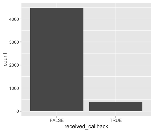
Notation
yi = whether a (fictitious) job candidate receives a call back.
πi = probability that the ith job candidate will receive a call back.
1−πi = probability that the ith job candidate will not receive a call back.
Where is the line?
ggplot(resume, aes(x = race, y = received_callback)) + geom_point()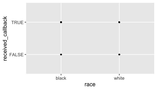
The Linear Model
We can model the probability of receiving a callback with a linear model.
transformation(πi)=β0+β1x1i+β2x2i+....βkxki
The Linear Model
We can model the probability of receiving a callback with a linear model.
transformation(πi)=β0+β1x1i+β2x2i+....βkxki
logit(πi)=β0+β1x1i+β2x2i+....βkxki
The Linear Model
We can model the probability of receiving a callback with a linear model.
transformation(πi)=β0+β1x1i+β2x2i+....βkxki
logit(πi)=β0+β1x1i+β2x2i+....βkxki
logit(πi)=log(πi1−πi)
The Linear Model
We can model the probability of receiving a callback with a linear model.
transformation(πi)=β0+β1x1i+β2x2i+....βkxki
logit(πi)=β0+β1x1i+β2x2i+....βkxki
logit(πi)=log(πi1−πi)
Note that log is natural log and not base 10. This is also the case for the log() function in R.
Probability πi Probability of receiving a callback.
Probability πi Probability of receiving a callback.
Odds πi1−πi Odds of receiving a callback.
Probability πi Probability of receiving a callback.
Odds πi1−πi Odds of receiving a callback.
Logit log(πi1−πi) Logit of receiving a callback.
When race is black (0)
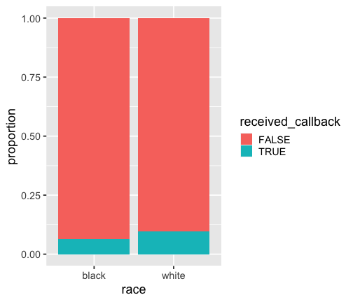
resume %>% filter(race == "black") %>% count(received_callback) %>% mutate(prop = n / sum(n))## # A tibble: 2 x 3## received_callback n prop## <lgl> <int> <dbl>## 1 FALSE 2278 0.936 ## 2 TRUE 157 0.0645Note that R assigns 0 an 1 to levels of categorical variables in alphabetical order. In this case black (0) and white(1)
When race is black (0)
p_b <- resume %>% filter(race == "black") %>% count(received_callback) %>% mutate(prop = n / sum(n)) %>% filter(received_callback == TRUE) %>% select(prop) %>% pull()Probability of receiving a callback when the candidate has a Black sounding name is 0.0644764.
When race is white (1)
p_w <- resume %>% filter(race == "white") %>% count(received_callback) %>% mutate(prop = n / sum(n)) %>% filter(received_callback == TRUE) %>% select(prop) %>% pull()Probability of receiving a callback when the candidate has a white sounding name is 0.0965092.
p_b## [1] 0.06447639## Oddsodds_b <- p_b / (1 - p_b)odds_b## [1] 0.06892011## Logitlogit_b <- log(odds_b)logit_b## [1] -2.674807p_b## [1] 0.06447639## Oddsodds_b <- p_b / (1 - p_b)odds_b## [1] 0.06892011## Logitlogit_b <- log(odds_b)logit_b## [1] -2.674807p_w## [1] 0.09650924## Oddsodds_w <- p_w / (1 - p_w)odds_w## [1] 0.1068182## Logitlogit_w <- log(odds_w)logit_w## [1] -2.236627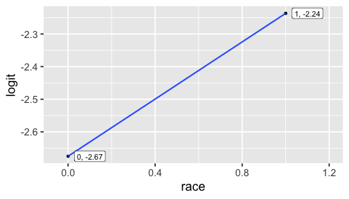
This is THE LINE of the linear model. As x increases by 1 unit, the expected change in the logit of receiving call back is 0.4381802. In this case, this is just the difference between logit for the white group and the black group.
The slope of the line is:
logit_w - logit_b## [1] 0.4381802The intercept is
logit_b## [1] -2.674807model_r <- glm(received_callback ~ race, data = resume, family = binomial)tidy(model_r)## # A tibble: 2 x 5## term estimate std.error statistic p.value## <chr> <dbl> <dbl> <dbl> <dbl>## 1 (Intercept) -2.67 0.0825 -32.4 1.59e-230## 2 racewhite 0.438 0.107 4.08 4.45e- 5log(^πi1−^πi)=−2.67+0.438×racewhitei
| Scale | Range |
|---|---|
| Probability | 0 to 1 |
| Odds | 0 to ∞ |
| Logit | - ∞ to ∞ |
We will consider years of experience as an explanatory variable. Normally, we would also include race in the model and have multiple explanatory variables, however, for learning purposes, we will keep the model simple.
model_y <- glm(received_callback ~ years_experience, data = resume, family = binomial)tidy(model_y)## # A tibble: 2 x 5## term estimate std.error statistic p.value## <chr> <dbl> <dbl> <dbl> <dbl>## 1 (Intercept) -2.76 0.0962 -28.7 5.58e-181## 2 years_experience 0.0391 0.00918 4.26 2.07e- 5model_y_summary <- tidy(model_y)intercept <- model_y_summary %>% filter(term == "(Intercept)") %>% select(estimate) %>% pull()slope <- model_y_summary %>% filter(term == "years_experience") %>% select(estimate) %>% pull()From logit to odds
Logit for a Candidate with 1 year of experience (rounded equation)
−2.76+0.0391×1
From logit to odds
Logit for a Candidate with 1 year of experience (rounded equation)
−2.76+0.0391×1
Odds for a Candidate with 1 year of experience
odds=elogit
πi1−πi=elog(πi1−πi)
^πi1−^πi=e−2.76+0.0391×1
From odds to probability
πi=odds1+odds
πi=πi1−πi1+πi1−πi
^πi=e−2.76+0.0391×11+e−2.76+0.0391×1=0.0618
Note you can use exp() function in R for exponentiating number e.
exp(1)## [1] 2.718282Logistic Regression model
Logit form:
log(πi1−πi)=β0+β1x1i+β2x2i+....βkxki
Probability form:
πi=eβ0+β1x1i+β2x2i+....βkxki1+eβ0+β1x1i+β2x2i+....βkxki
Estimated probability of a candidate with 0 years of experience receiving a callback
^πi=e−2.76+0.0391×01+e−2.76+0.0391×0=0.0595
Estimated probability of a candidate with 1 year of experience receiving a callback
^πi=e−2.76+0.0391×11+e−2.76+0.0391×1=0.0618
model_ryc <- glm(received_callback ~ race + years_experience + job_city, data = resume, family = binomial)tidy(model_ryc)## # A tibble: 4 x 5## term estimate std.error statistic p.value## <chr> <dbl> <dbl> <dbl> <dbl>## 1 (Intercept) -2.78 0.134 -20.8 6.18e-96## 2 racewhite 0.440 0.108 4.09 4.39e- 5## 3 years_experience 0.0332 0.00940 3.53 4.11e- 4## 4 job_cityChicago -0.329 0.108 -3.04 2.33e- 3The estimated probability that a Black candidate with 10 years of experience, residing in Boston, would receive a callback.
^πi=e−2.78+(0.0440×0)+(0.0332×10)+(−0.0329×0)1+e−2.78+(0.0440×0)+(0.0332×10)+(−0.0329×0)=0.0796
We have used the data for educational purposes. The original study considers many other variables that may influence whether someone receives a callback or not. Read the original study for other considerations.