class: title-slide <br> <br> .pull-right[ # Simple Linear Regression ## Dr. Mine Dogucu ] --- #### Data `babies` in `openintro` package ``` ## Rows: 1,236 ## Columns: 8 ## $ case <int> 1, 2, 3, 4, 5, 6, 7, 8, 9, 10, 11, 12, 13, 14, 15, 16, 17, 1… ## $ bwt <int> 120, 113, 128, 123, 108, 136, 138, 132, 120, 143, 140, 144, … ## $ gestation <int> 284, 282, 279, NA, 282, 286, 244, 245, 289, 299, 351, 282, 2… ## $ parity <int> 0, 0, 0, 0, 0, 0, 0, 0, 0, 0, 0, 0, 0, 0, 0, 0, 0, 0, 0, 0, … ## $ age <int> 27, 33, 28, 36, 23, 25, 33, 23, 25, 30, 27, 32, 23, 36, 30, … ## $ height <int> 62, 64, 64, 69, 67, 62, 62, 65, 62, 66, 68, 64, 63, 61, 63, … ## $ weight <int> 100, 135, 115, 190, 125, 93, 178, 140, 125, 136, 120, 124, 1… ## $ smoke <int> 0, 0, 1, 0, 1, 0, 0, 0, 0, 1, 0, 1, 1, 1, 0, 0, 1, 1, 0, 1, … ``` --- ## Baby Weights .pull-left[ ```r ggplot(babies, aes(x = gestation, y = bwt)) + geom_point() ``` ] .pull-right[ <img src="09a-slr_files/figure-html/unnamed-chunk-4-1.png" style="display: block; margin: auto;" /> ] --- ## Baby Weights .pull-left[ ```r ggplot(babies, aes(x = gestation, y = bwt)) + geom_point() + geom_smooth(method = "lm", se = FALSE) ``` `lm` stands for linear model `se` stands for standard error ] .pull-right[ <img src="09a-slr_files/figure-html/unnamed-chunk-6-1.png" style="display: block; margin: auto;" /> ] --- class: middle <div align = "center"> | y | Response | Birth weight | Numeric | |---|-------------|-----------------|---------| | x | Explanatory | Gestation | Numeric | --- ## Linear Equations Review .pull-left[ Recall from your previous math classes `\(y = mx + b\)` where `\(m\)` is the slope and `\(b\)` is the y-intercept e.g. `\(y = 2x -1\)` ] -- .pull-right[ <!-- --> Notice anything different between baby weights plot and this one? ] --- class: middle .pull-left[ **Math** class `\(y = b + mx\)` `\(b\)` is y-intercept `\(m\)` is slope ] .pull-left[ **Stats** class `\(y_i = \beta_0 +\beta_1x_i + \epsilon_i\)` `\(\beta_0\)` is y-intercept `\(\beta_1\)` is slope `\(\epsilon_i\)` is error/residual `\(i = 1, 2, ...n\)` identifier for each point ] --- ```r model_g <- lm(bwt ~ gestation, data = babies) ``` `lm` stands for linear model. We are fitting a linear regression model. Note that the variables are entered in y ~ x order. --- ```r broom::tidy(model_g) ``` ``` ## # A tibble: 2 x 5 ## term estimate std.error statistic p.value ## <chr> <dbl> <dbl> <dbl> <dbl> ## 1 (Intercept) -10.1 8.32 -1.21 2.27e- 1 ## 2 gestation 0.464 0.0297 15.6 3.22e-50 ``` -- `\(\hat {y}_i = b_0 + b_1 x_i\)` `\(\hat {\text{bwt}_i} = b_0 + b_1 \text{ gestation}_i\)` `\(\hat {\text{bwt}_i} = -10.1 + 0.464\text{ gestation}_i\)` --- class: middle ## Expected bwt for a baby with 300 days of gestation `\(\hat {\text{bwt}_i} = -10.1 + 0.464\text{ gestation}_i\)` `\(\hat {\text{bwt}} = -10.1 + 0.464 \times 300\)` `\(\hat {\text{bwt}} =\)` 129.1 For a baby with 300 days of gestation the expected birth weight is 129.1 ounces. --- ## Interpretation of estimates .pull-left[ <img src="09a-slr_files/figure-html/unnamed-chunk-10-1.png" style="display: block; margin: auto;" /> `\(b_1 = 0.464\)` which means for one unit(day) increase in gestation period the expected increase in birth weight is 0.464 ounces. ] -- .pull-right[ <img src="09a-slr_files/figure-html/unnamed-chunk-11-1.png" style="display: block; margin: auto;" /> `\(b_0 = -10.1\)` which means for gestation period of 0 days the expected birth weight is -10.1 ounces!!!!!!!! (does NOT make sense) ] --- class: middle ## Extrapolation - There is no such thing as 0 days of gestation. -- - Birth weight cannot possibly be -10.1 ounces. -- - Extrapolation happens when we use a model outside the range of the x-values that are observed. After all, we cannot really know how the model behaves (e.g. may be non-linear) outside of the scope of what we have observed. --- ## Baby number 148 .pull-left[ ```r babies %>% filter(case == 148) %>% select(bwt, gestation) ``` ``` ## # A tibble: 1 x 2 ## bwt gestation ## <int> <int> ## 1 160 300 ``` ] .pull-right[ <!-- --> ] --- ## Baby #148 .pull-left[ **Expected** `\(\hat y_{148} = b_0 +b_1x_{148}\)` `\(\hat y_{148} = -10.1 + 0.464\times300\)` `\(\hat y_{148}\)` = 129.1 ] .pull-left[ **Observed** `\(y_{148} =\)` 160 ] --- ## Residual for `i = 148` .pull-left[ <img src="09a-slr_files/figure-html/unnamed-chunk-14-1.png" style="display: block; margin: auto;" /> ] .pull-right[ `\(y_{148} = 160\)` <hr> `\(\hat y_{148}\)` = 129.1 <hr> `\(e_{148} = y_{148} - \hat y_{148}\)` `\(e_{148} =\)` 30.9 ] --- ## Least Squares Regression The goal is to minimize `$$e_1^2 + e_2^2 + ... + e_n^2$$` -- which can be rewritten as `$$\sum_{i = 1}^n e_i^2$$` --- ## Conditions for Least Squares Regression - Linearity - Normality of Residuals - Constant Variance - Independence --- .pull-left[ .center[**Linear**] <!-- --> ] .pull-right[ .center[**Non-linear**] <!-- --> ] --- .pull-left[ .center[**Nearly normal**] 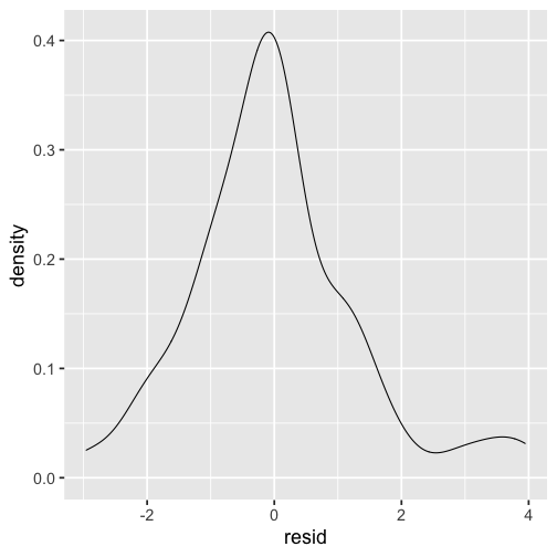<!-- --> ] .pull-right[ .center[**Not normal**] 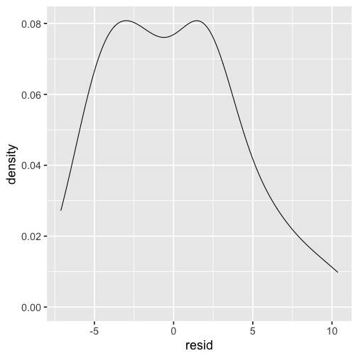<!-- --> ] --- .pull-left[ .center[**Constant Variance**] 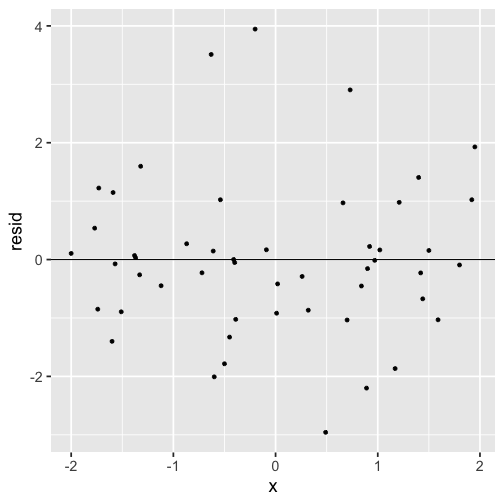<!-- --> ] .pull-right[ .center[**Non-constant variance**] 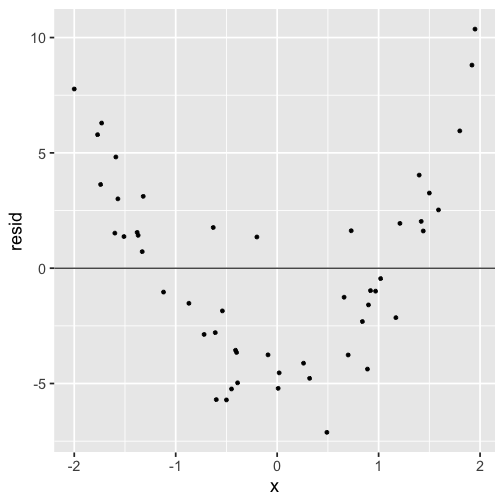<!-- --> ] --- class: middle ## Independence Harder to check because we need to know how the data were collected. -- In the description of the dataset it says _[a study]considered all pregnancies between 1960 and 1967 among women in the Kaiser Foundation Health Plan in the San Francisco East Bay area._ -- It is possible that babies born in the same hospital may have similar birth weight. -- Correlated data examples: patients within hospitals, students within schools, people within neighborhoods, time-series data. --- class: middle ### Inference: Confidence Interval ```r confint(model_g) ``` ``` ## 2.5 % 97.5 % ## (Intercept) -26.3915884 6.2632199 ## gestation 0.4059083 0.5226169 ``` Note that the confidence interval for the slope does not contain zero and all the values in the interval are positive indicating a possible positive relationship between gestation and birth weight.